A Multiverse Reanalysis of Likert-Type Responses

Abstract

There is no consensus on how to best analyze responses to single Likert items. Therefore, studies involving Likert-type responses can be perceived as untrustworthy by researchers who disagree with the particular statistical analysis method used. We report a multiverse reanalysis of such a study, consisting of nine different statistical analyses. The conclusions are consistent with the previously reported findings, and are remarkably robust to the choice of statistical analysis.

Author Keywords

Likert data; explorable explanation; multiverse analysis.

ACM Classification Keywords

H5.2 User Interfaces: Evaluation/Methodology

General Terms

Human Factors; Design; Experimentation; Measurement.

Introduction

In 2014, Tal and Wansink published a study entitled "Blinded with science: Trivial graphs and formulas increase ad persuasiveness and belief in product efficacy" in the journal Public Understanding of Science. The study shows that adding a chart to a statement about a new drug increases people's belief in the drug's efficacy. However, a 2016 replication by Dragicevic and Jansen suggests that the effect may not be as robust as claimed: in a series of four replications conducted on two crowdsourcing platforms, the chart appeared to be no more persuasive – and sometimes less persuasive – than text alone.

However, these results are based on Likert-type responses, which are known to be tricky to analyze, as there is currently no consensus on how to best analyze this type of data. Tal and Wansink used simple t-tests, while Dragicevic and Jansen used bootstrap confidence intervals in order to gain more robustness against possible departures from the normality assumption. However, there are many other ways the same data could have been analyzed. Here we report on nine different ways of analyzing the data. All these methods lead to the same conclusions, confirming that the findings are robust to the choice of statistical analysis.

Our reporting approach which combines the principle of multiverse analysis with the idea of explorable explanation can be used not only in reanalyses but also in original studies in order to make findings results more reliable and more convincing when there is a disagreement about the best statistical analysis method.

Dataset and Questions

Dragicevic and Jansen's study has four experiments. In each experiment, each participant is either shown a text about a hypothetical drug ("no_graph" condition) or the same text with a chart ("graph" condition). The participant is then asked to assess to what extent the drug is effective, on a scale from 1 to 7. We focus on this data here. The study has another important dependent variable (error of the response to a comprehension question) but it is not Likert-type data and therefore not addressed here.

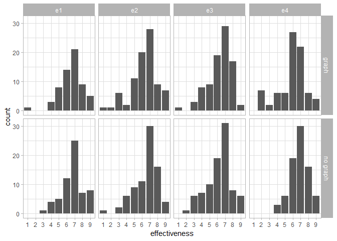
Figure 1 shows the distribution of the raw data. Our question is whether there is an overall difference between graph and no_graph, for each of the four experiments (e1 to e4). We answer this question using nine different statistical analyses, whose results are summarized in the next section.

Summary of Results

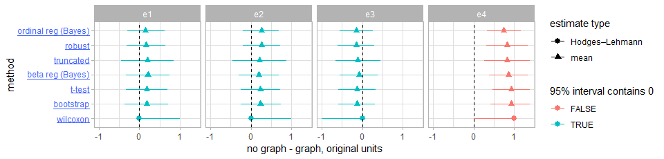
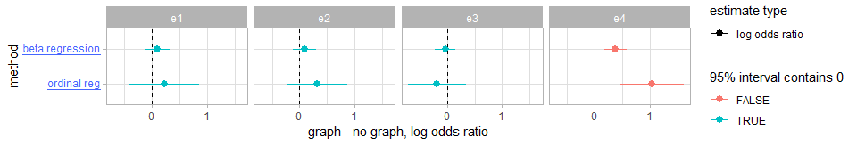
Seven of the nine methods provide us with a point estimate and a 95% interval estimate of the average difference between the two conditions, all summarized in Figure 2. The remaining two procedures provide estimates as a log-odds ratio, shown in Figure 3 (for beta regression, this is the log of the ratio of the odds of going from one extreme of the scale to the other between the two conditions; for ordinal regression, this is the log of the ratio of the odds of going from one category on the scale to any category above it between the two conditions; 0 indicates equal odds). On both figures, red intervals are statistically significant at the .05 level, while blue intervals are non-significant.

Click on an analysis label to see its details in the next section. The complete source code of all analyses is available at R/analysis.html.

Analysis Details

Tal and Wansink used a t-test to analyze their own data. For this method, we compute the difference between the two means, its 95% t-based confidence interval for independent samples and the corresponding p-value for a null hypothesis of no effect. This method assumes normal sampling distributions, which is reasonable here given that the data is bell-shaped and sample sizes range between N=60 and N=90 per condition. Dragicevic and Jansen analyzed their data using the bootstrap method. With this method, we compute the 95% BCa non-parametric bootstrap confidence interval for the difference between two means. Bootstrapping has been shown to work with a range of exotic data distributions but can give liberal interval estimates when the sample size is small (i.e., N ≤ 10, which is not the case here since sample sizes range between N=60 and N=90 per condition). This method does not provide a p-value. For the wilcoxon method, we use a Wilcoxon signed-rank test and compute the corresponding p-value for a null hypothesis of no effect. The Wilcoxon signed-rank test is a non-parametric method commonly recommended as an alternative to the t-test when there are reasons to doubt the normality assumption. The estimate (and its 95% CI) are for the median of the difference between samples (not the difference in the medians). For the beta regression method, we perform a maximum-likelihood regression with a beta-distributed dependent variable. This method has been recommended for analyzing scales with a lower and upper bound and is robust to skew and heteroscedasticity . We rescaled the data to be in (0, 1) by dividing all responses by 10. We report the log odds ratio between conditions: the log of the ratio of the odds of going from one extreme of the scale to the other. For the beta reg (Bayes) method, we use a Bayesian formulation of beta regression. This method has been recommended for analyzing scales with a lower and upper bound and is robust to skew and heteroscedasticity . We rescaled the data to be in (0, 1) by dividing all responses by 10. We fit a beta regression within each experiment, using weakly informative priors. We report estimates of marginal means on the original scale. For the ordinal reg method, we use an ordinal logistic regression . Ordinal models are often applied to Likert-type data. We report the log odds ratio between conditions: the log of the ratio of the odds of going from one category on the scale to any category above it. For the ordinal reg (Bayes) method, we use a Bayesian ordinal logistic regression . Ordinal models are often applied to Likert-type data. We report estimates of marginal means on the original scale. For the robust method, we perform a robust, heteroskedastic linear regression: we use a Student t error distribution instead of Gaussian error distribution, and estimate a different variance parameter for each group. This is essentially Kruschke's BEST test (a Bayesian, robust, hetereoskedastic alternative to the t-test), but estimated using a frequentist procedure instead of a Bayesian one. For the truncated method, we perform a truncated normal regression model. This model also accounts for hetereoskedasticity (non-constant variance) by estimating a different variance parameter for each condition.

The point estimate of the mean difference and its 95% confidence interval are reported in Figure 2, for each of the four experiments (row labeled ttest). According to the t-tests, there is no evidence for a difference on average between graph and no_graph, except for experiment 4, for which there is strong evidence for an effect in the opposite direction (no_graph more persuasive than graph, p=.00013). The point estimate of the mean difference and its 95% confidence interval are reported in Figure 2, for each of the four experiments (row labeled bootstrap). According to the bootstrap procedure, there is no evidence for a difference on average between graph and no_graph, except for experiment 4, for which there is strong evidence for an effect in the opposite direction (no_graph more persuasive than graph). The point estimate of the mean difference and its 95% confidence interval are reported in Figure 2, for each of the four experiments (row labeled wilcoxon). According to the Wilcoxon tests, there is no evidence for a difference on average between graph and no_graph, except for experiment 4, for which there is strong evidence for an effect in the opposite direction (no_graph more persuasive than graph, p=.00040). The log-odds ratio and its 95% confidence interval are reported in Figure 3, for each of the four experiments (first row). According to the beta regressions, there is no evidence for a difference on average between graph and no_graph, except for experiment 4, for which there is strong evidence for an effect in the opposite direction (no_graph more persuasive than graph, p=.00017). The point estimate of the mean difference and its 95% posterior quantile interval are reported in Figure 2, for each of the four experiments (row labeled beta reg (Bayes)). According to the beta regressions, there is no evidence for a difference on average between graph and no_graph, except for experiment 4, for which there is strong evidence for an effect in the opposite direction (no_graph more persuasive than graph). The log-odds ratio and its 95% confidence interval are reported in Figure 3, for each of the four experiments (second row). According to the ordinal regressions, there is no evidence for a difference on average between graph and no_graph, except for experiment 4, for which there is strong evidence for an effect in the opposite direction (no_graph more persuasive than graph, p=.00040). The point estimate of the mean difference and its 95% posterior quantile interval are reported in Figure 2, for each of the four experiments (row labeled ordinal reg (Bayes)). According to the ordinal regressions, there is no evidence for a difference on average between graph and no_graph, except for experiment 4, for which there is strong evidence for an effect in the opposite direction (no_graph more persuasive than graph). The point estimate of the mean difference and its 95% confidence interval are reported in Figure 2, for each of the four experiments (row labeled robust). According to the robust linear regressions, there is no evidence for a difference on average between graph and no_graph, except for experiment 4, for which there is strong evidence for an effect in the opposite direction (no_graph more persuasive than graph, p=.00016). The point estimate of the mean difference and its 95% confidence interval are reported in Figure 2, for each of the four experiments (row labeled truncated). According to the truncated normal regressions, there is no evidence for a difference on average between graph and no_graph, except for experiment 4, for which there is strong evidence for an effect in the opposite direction (no_graph more persuasive than graph, p=.00037).

For information on any of the other eight statistical analyses we conducted, click on its label on Figure 2 or Figure 3.

Discussion

However we analyze the data, the substantive conclusions are about the same. While the Wilcoxon estimates and intervals in Figure 1 look different from the other estimates, it is estimating a slightly different quantity: a median of the differences instead of a difference in means (as the other approaches in Figure 2 are). In Figure 3, while the two rows are both on the log odds scale, they are measuring log odds ratios of different things, so it is hard to compare the values directly. Since the ordinal regression measures the log odds ratio of an increase from one category to any category above it, we should expect this value to be larger than the estimate from the beta regression, which measures the log odds ratio of going from one extreme of the scale to the other (a less likely event). With smaller sample sizes, it is likely that the results would have differed more.

From this multiverse analysis, we can conclude that our results are very robust, and not strongly sensitive to the choice of analysis method: if the conclusions of Dragicevic and Jansen were to be wrong, it is very unlikely that the cause would be in the choice of statistical analysis.

Our reporting approach, which combines the principle of multiverse analysis with the idea of explorable explanation , can be used not only in reanalyses but also in original studies in order to make statistical results more convincing when there is no consensus as to what method is best to analyze such data.